We now provide how to replicate a simulation analysis using tresor, a tool for simulating sequencing reads, for a previously published method for alleviating errors during bead synthesis. The goal is to investigate how modifications to beads used in single-cell sequencing can improve the recognition of unique molecular identifiers (UMIs) and cell barcodes in long-read sequencing data.
Please read this tutorial for some technical bases.
1. Install Tresor and UMIche
We first install Tresor (version 0.1.1).
# create a conda environment
conda create --name tresor python=3.11

# activate the conda environment
conda activate tresor

pip install tresor==0.1.1
After that, we can install UMIche (version 0.1.5) to assist with the analysis of reads generated by tresor.
pip install umiche==0.1.52. Read simulation
2.1 Error types
Next, we need to define several simulation scenarios, all related to sequencing errors:
- PCR deletion
- PCR insertion
- Sequencing insertion
- Sequencing deletion
2.2 Basic settings
Import two libraries, Tresor and UMIche.
import tresor as ts
import umiche as uc
For each simulation scenario, we generate sequencing reads (beads) under 17 different error rates (criteria).
criteria = [
    1e-05,
    2.5e-05,
    5e-05,
    7.5e-05,
    0.0001,
    0.00025,
    0.0005,
    0.00075,
    0.001,
    0.0025,
    0.005,
    0.0075,
    0.01,
    0.025,
    0.05,
    0.075,
    0.1,
]
The simulation is executed over 10 independent permutations, with each permutation varying key error parameters and random seeds to test reproducibility and robustness. For each permutation, a set of PCR deletion rate criteria (criteria) is tested in turn.
permutation_times = 102.3 Structure configuration
After that, we can use the following function to generate the sequencing reads.
Our design mimics real-world bead-bound oligonucleotide structures used in single-cell platforms like 10x Genomics. Read components are flexibly placed in certain order, added, and/or removed through len_params. There are two types of barcodes, a 12UMI (umi) with a homodimer unit (2-mer) a 12 bp cell barcode. Other sequence elements (seq_params) includes 3 custom adapter-like motifs:
- A 4 bp anchor (
custom_1='BAGC'), and two tail sequences: - A 1 bp linker (
custom_2='A') - A 30 bp polyT tail (
custom_3='TTT...T')
The anchor is interposed between the barcode and the UMI to serve as a landmark for parsing reads in downstream analysis.
2.4 Simulation conditions
It initially generates 50 sequences (seq_num=50) of length 100 bp (seq_len=100) per condition. FastQ files are saved in a structured directory tree based on permutation index (permute_0, permute_1, etc.). It uses condis to specify the ordered structure of the synthetic molecule from custom adapter to polyT tail, including the anchor and UMI. It simulates errors during both PCR amplification and sequencing, including deletions and insertions with specific rates (e.g., pcr_del_rate=criterion and pcr_ins_rate=7.1e-7). The substitution error rate is set to (seq_error=0.001). The error distribution model is nbinomial to simulate the distribution of PCR errors. It ensures reproducibility with fixed random seeds (seed=permut_i).
2.5 File type
Output files are stored and named systematically for further parsing and statistical comparison (e.g., pcr_del_0.fastq, pcr_del_1.fastq, etc.).
2.6 Running
We can run the following code to generate the reads.
for permut_i in range(permutation_times):
    for i, criterion in enumerate(criteria):
        ts.locus.simu_generic(
            len_params={
                'umi': {
                    'umi_unit_pattern': 2,
                    'umi_unit_len': 8,
                },
                'barcode': 12,
                'adapter': 12,
            },
            seq_params={
                'custom': 'TCTCTCTCTACACGACGCTCTTCCGATCT',  # length 29
                'custom_1': 'BAGC',  # length 4
                'custom_2': 'A',  # length 1
                'custom_3': 'T' * 30,  # length 30
            },
            seq_num=50,
            seq_len=100,
            working_dir='../../data/tresor/simu/pcr_del/permute_' + str(permut_i) + '/',
            fasta_cdna_fpn=False,
            # fasta_cdna_fpn=to('data/Homo_sapiens.GRCh38.cdna.all.fa.gz'),

            is_sv_umi_lib=True,
            is_sv_seq_lib=True,
            is_sv_primer_lib=True,
            is_sv_adapter_lib=True,
            is_sv_spacer_lib=True,
            condis=['custom', 'adapter', 'custom_1', 'umi', 'custom_2', 'custom_3'],
            sim_thres=3,
            permutation=permut_i,

            # PCR amplification
            ampl_rate=0.9,
            err_route='sptree',  # tree minnow err1d err2d mutation_table_minimum mutation_table_complete
            # pcr_error=criterion,
            pcr_error=1e-05,
            pcr_num=8,
            err_num_met='nbinomial',
            # seq_error=criterion,
            seq_error=0.001,
            seq_sub_spl_number=5000,  # None 200
            # seq_sub_spl_numbers=[5000],  # None 200
            # seq_sub_spl_numbers=[100, 500, 1000, 10000],  # None 200
            # seq_sub_spl_rate=0.333,

            pcr_deletion=True,  # True False
            pcr_insertion=True,
            pcr_del_rate=criterion, # 0.016 0.00004
            # pcr_ins_rate=criterion,
            pcr_ins_rate=7.1e-7, # 0.011 0.00001
            seq_deletion=True,
            seq_insertion=True,
            seq_del_rate=2.4e-6,
            seq_ins_rate=7.1e-7,
            # seq_ins_rate=7.1e-7,

            use_seed=True,
            seed=permut_i,

            verbose=False,  # True False

            sv_fastq_fp='../../data/tresor/simu/pcr_del/permute_' + str(permut_i) + '/',
            sv_fastq_fn="pcr_del_" + str(i),
        )
2.7 Output files
Figure 1:FastQ reads.
3. Analysis
Next comes the analysis phase, where we primarily use UMIche to identify reads that contain the anchor sequence. Since the sequencing data was generated under different PCR deletion error rates, we first define the following simulation scenarios.
scenario='pcr_del',
# scenario='seq_del',
# scenario='seq_ins',
# scenario='pcr_ins',
After that, we need to define additional parameters to enable the UMIche tool to perform accurate identification. The parameters are placed in a .yml file.
work_dir: ../../data/tresor/anchor/simu/pcr_del/

fixed:
  permutation_num: 10

varied:
    criteria: [
        1e-05,
        2.5e-05,
        5e-05,
        7.5e-05,
        0.0001,
        0.00025,
        0.0005,
        0.00075,
        0.001,
        0.0025,
        0.005,
        0.0075,
        0.01,
        0.025,
        0.05,
        0.075,
        0.1,
        # 0.2,
        # 0.3,
    ]

anchor:
    seq1: 'BAGC'
Next, we can use the following code to identify the anchor sequence and examine the percentage of captured reads under each permutation test.
pct_reads, pct_anchor_reads = uc.pipeline.anchor(
    scenario='pcr_del',
    param_fpn='../../data/tresor/anchor/params_anchor.yml',
)
Without anchor
{0: [0.9952, 0.9962, 0.9954, 0.9944, 0.9894, 0.9852, 0.9798, 0.9706, 0.9392, 0.8288, 0.771, 0.6808, 0.6126, 0.3122, 0.142, 0.0572, 0.0282], 1: [0.998, 0.9892, 0.9956, 0.9734, 0.978, 0.987, 0.953, 0.9536, 0.9346, 0.9046, 0.8136, 0.7044, 0.5678, 0.3194, 0.094, 0.0358, 0.0324], 2: [0.9972, 0.9956, 0.9956, 0.9948, 0.9702, 0.9614, 0.9672, 0.9506, 0.9042, 0.851, 0.7844, 0.6466, 0.5246, 0.2814, 0.0998, 0.061, 0.0232], 3: [0.9868, 0.9954, 0.994, 0.9956, 0.995, 0.9866, 0.936, 0.9348, 0.95, 0.8762, 0.7068, 0.6174, 0.6248, 0.27, 0.1254, 0.0608, 0.0286], 4: [0.9974, 0.9942, 0.9956, 0.994, 0.988, 0.9632, 0.9546, 0.9348, 0.9498, 0.8892, 0.7662, 0.666, 0.5966, 0.2898, 0.1236, 0.059, 0.0212], 5: [0.9964, 0.996, 0.9922, 0.9936, 0.9914, 0.9666, 0.975, 0.9622, 0.9758, 0.84, 0.7312, 0.6896, 0.5448, 0.2692, 0.0928, 0.0482, 0.0236], 6: [0.996, 0.994, 0.9926, 0.9812, 0.993, 0.9804, 0.9444, 0.9674, 0.9678, 0.8592, 0.782, 0.6528, 0.6428, 0.282, 0.118, 0.0584, 0.0386], 7: [0.9966, 0.9962, 0.9958, 0.9932, 0.9914, 0.9822, 0.9346, 0.9442, 0.9306, 0.8476, 0.8036, 0.697, 0.6026, 0.3232, 0.1032, 0.0376, 0.0272], 8: [0.997, 0.995, 0.9928, 0.9938, 0.9922, 0.988, 0.984, 0.9636, 0.9426, 0.9036, 0.7962, 0.6374, 0.5552, 0.2944, 0.0866, 0.0422, 0.0256], 9: [0.9962, 0.991, 0.9956, 0.9928, 0.9928, 0.9856, 0.9802, 0.9528, 0.9366, 0.9044, 0.7412, 0.7106, 0.5484, 0.3078, 0.1202, 0.0418, 0.0264]}With anchor
{0: [0.981, 0.9402, 0.9622, 0.8878, 0.8486, 0.6536, 0.4906, 0.3792, 0.287, 0.0862, 0.0192, 0.003, 0.0008, 0.0, 0.0, 0.0, 0.0], 1: [0.9938, 0.9716, 0.9328, 0.8968, 0.868, 0.7362, 0.5006, 0.393, 0.2776, 0.0768, 0.0072, 0.003, 0.0018, 0.0, 0.0, 0.0, 0.0], 2: [0.994, 0.974, 0.917, 0.9164, 0.8914, 0.6954, 0.5458, 0.3634, 0.297, 0.0644, 0.009, 0.0026, 0.001, 0.0, 0.0, 0.0, 0.0], 3: [0.9766, 0.969, 0.9596, 0.8992, 0.9014, 0.6024, 0.448, 0.3616, 0.2564, 0.0862, 0.0062, 0.0038, 0.0006, 0.0002, 0.0, 0.0, 0.0], 4: [0.9898, 0.9668, 0.9068, 0.8852, 0.849, 0.7704, 0.546, 0.3638, 0.318, 0.0866, 0.016, 0.0038, 0.0014, 0.0002, 0.0, 0.0, 0.0], 5: [0.9952, 0.9688, 0.9598, 0.9166, 0.8304, 0.6936, 0.4916, 0.4086, 0.316, 0.0704, 0.013, 0.0046, 0.0014, 0.0, 0.0, 0.0, 0.0], 6: [0.9678, 0.981, 0.927, 0.928, 0.865, 0.7012, 0.5252, 0.4332, 0.2636, 0.092, 0.0126, 0.0022, 0.0006, 0.0, 0.0, 0.0, 0.0], 7: [0.9836, 0.9562, 0.9226, 0.8764, 0.876, 0.726, 0.5374, 0.3614, 0.3218, 0.058, 0.0146, 0.0042, 0.0014, 0.0, 0.0, 0.0, 0.0], 8: [0.9778, 0.9614, 0.9366, 0.9046, 0.8822, 0.7604, 0.5196, 0.3692, 0.2664, 0.0648, 0.0108, 0.003, 0.0014, 0.0, 0.0, 0.0, 0.0], 9: [0.9972, 0.9696, 0.966, 0.908, 0.9056, 0.7056, 0.5192, 0.3878, 0.2856, 0.067, 0.013, 0.0036, 0.0018, 0.0, 0.0, 0.0, 0.0]}4. Visualisation
We use the following code to generate the plot. This function visualizes the anchor detection efficiency by plotting the percentage of total reads captured and the percentage of anchor-containing reads across different error rates. You can switch the condition argument to analyze other types of error scenarios.
uc.vis.anchor_efficiency(
    criteria=criteria,
    quant_captured=pct_reads,
    quant_anchor_captured=pct_anchor_reads,
    condition='PCR deletion error rate',
    # condition='Sequencing deletion error rate',
    # condition='Sequencing insertion error rate',
    # condition='PCR insertion error rate',
)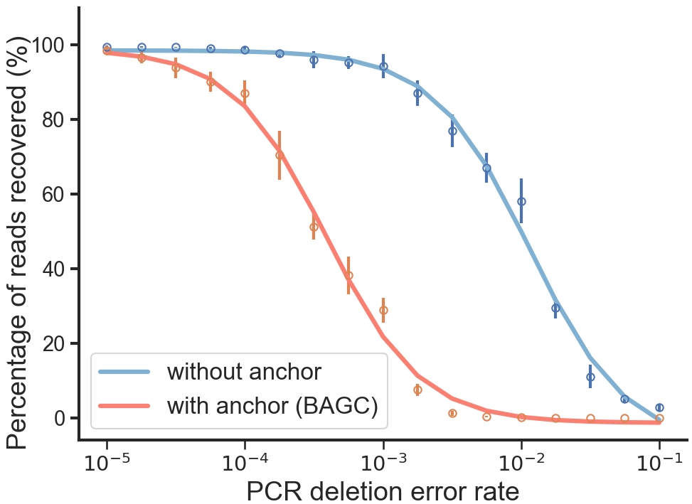
Figure 2:Percentage of captured reads with or without an anchor.
In addition, we can use the following code to visualise it with bars.
uc.vis.anchor_efficiency_simple(
    criteria=criteria,
    quant_captured=pct_reads,
    quant_anchor_captured=pct_anchor_reads,
    condition='PCR deletion error rate',
    # condition='Sequencing deletion error rate',
    # condition='Sequencing insertion error rate',
    # condition='PCR insertion error rate',
)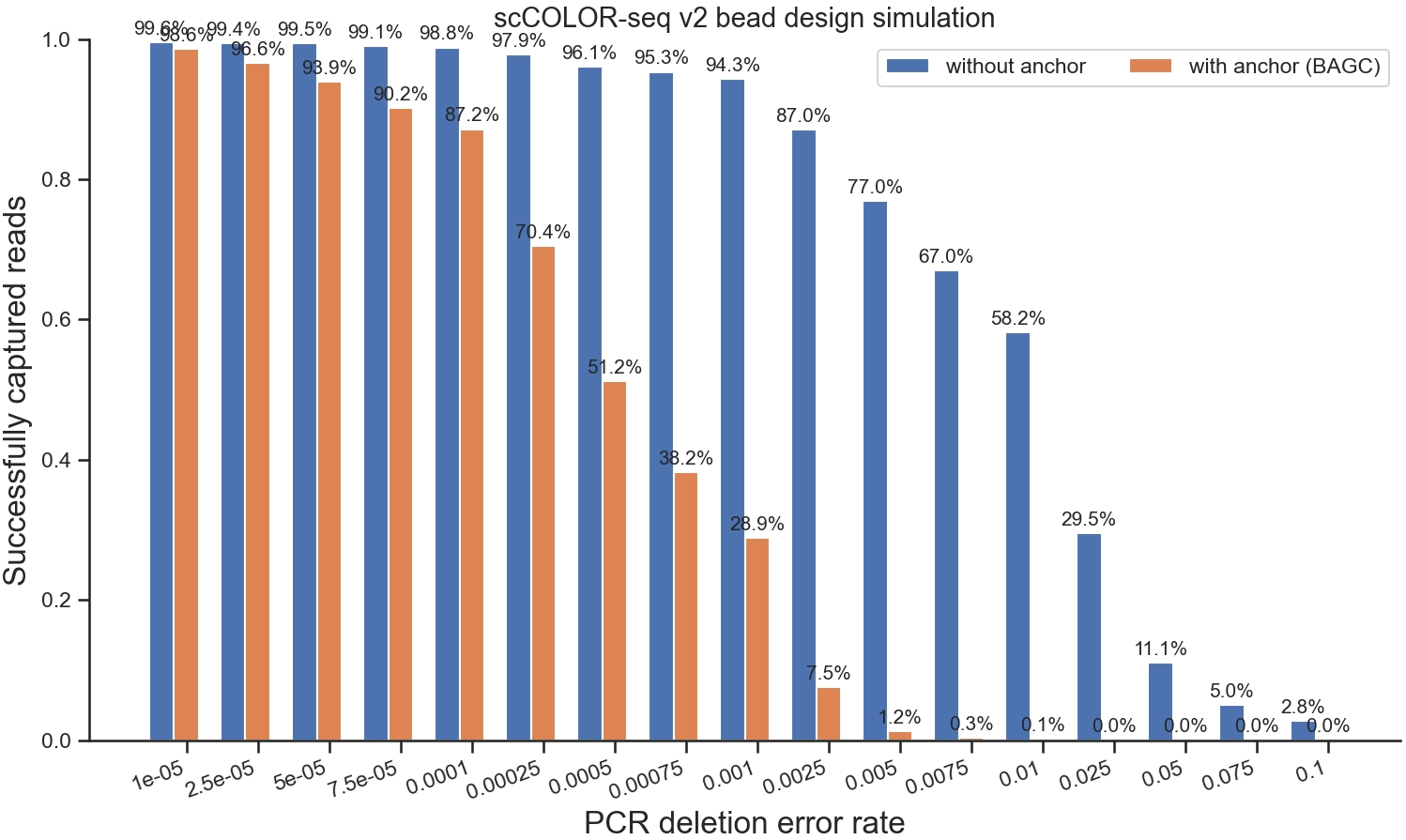
Figure 3:Percentage of captured reads with or without an anchor.